1. Introduction
2. The SIR epidemic model
2.1. The stochastic SIR epidemic model
3. The SHAR modelling framework
4. The SHARUCD model framework
4.1. Modeling the effects of the control measures (first wave)
4.2. Model simulations with control and data
4.3. Model Validation and short-term prediction exercise with control measure
4.4. Growth rates and reproduction ratio
5. The refined SHARUCD MODEL with import and seasonality (second phase)
5.1. Model simulations and short term predictions
5.2. Short term predictions of COVID-19 in the Basque Country
6. Acknowledgments and contributions
7. References

1. Introduction:

In December 2019, a new respiratory syndrome (COVID-19) caused by a new coronavirus (SARS-CoV-2), was identified in China [1] and spread rapidly around the globe. COVID-19 was declared a pandemic by the World Health Organization (WHO) in March, 2020 [2]. By the end of December, 2021, more than 280 million cases were confirmed with more than 5.4 million deaths [3].

Following evaluation by the European Medicines Agency (EMA), the following vaccines can be used in the EU to prevent COVID-19:

BioNTech and Pfizer (mRNA, 2 doses)
Moderna (mRNA, 2 doses)
AstraZeneca (adenovirus, 2 doses)
Johnson & Johnson/Janssen Pharmaceuticals (adenovirus, 1 dose)
Novavax (protein, 2 doses):

Moreover, several other vaccines are at different stages of assessment by the EMA [4,5].

Different COVID-19 vaccine efficacy are reported, with remarkable effectiveness against severe disease. The so called sterilizing immunity, occurring when vaccinated individuals cannot transmit the virus, is still being evaluated. It is also unclear to what extent people with no symptoms or mild infection transmit the disease, and estimating their contribution to outbreaks is challenging. Note that vaccine efficacy is changing overtime, and might depend on dosage and COVID-19 variants.

COVID-19 situation worldwide, as of January 6, 2022

Figure 1: COVID-19 cases, death and vaccination worldwide. In a) confirmed cases, in b) deceased cases and in c) cumulative vaccine doses administrated and in d) daily new vaccinations around the globe. As of January 6, 2022, a total of 296.496.809 positive cases and 5.462.631 deaths were reported worldwide. 9.118.223.397 vaccine doses were administered, with 4.567.405 833 persons vaccinated with at least one dose and 3.864.889.174 persons fully vaccinated [6].

In March 2020, a Multidisciplinary Task Force (so-called Basque Modelling Task Force, BMTF) was created to assist the Basque Health managers and the Basque Government during the COVID-19 responses. BMTF is a modeling team, working on different approaches, including stochastic processes, statistical methods and artificial intelligence. Members were collaborating taking into consideration all information provided by the public health frontline and using different available datasets in respect to the COVID-19 outbreak in the Basque Country. The objectives were, besides projections on the national health system’s necessities during the increased population demand on hospital admissions, the description of the epidemic in terms of disease spreading and control, as well as monitoring the disease transmission when the country lockdown was gradually lifted. All modeling approaches are complementary and are able to provide coherent results, assuring that the decisions made using the modeling results were sound and, in fact, adjusted to the current epidemiological data.

In this dashboard we describe and present the results obtained by the modeling approach developed by the Mathematical and Theoretical Biology (MTB) group at BCAM, within the BMTF initiative. We developed a flexible stochastic SHAR (susceptible (S), severe cases prone to hospitalization (H), mild, sub-clinical or asymptomatic (A), recovered (R)) framework, an extension of the basic epidemiological SIR-type model.

We start presenting the properties of the basic SIR epidemic model for infectious diseases [7,8], with the goal to introduce notation, terminology, and results that will be generalized in later sections on more advanced models describing the COVID-19 epidemiology. This dashboard will be updated every month.

2. The SIR epidemic model:

The simple SIR model (susceptible-infected-recovered) model is one of the simplest compartmental models, dividing the observed population into three groups: the class S of susceptible individuals to the considered disease, the class of infected individuals I, and the class R of individuals who have recovered from the infection. In analogy with chemical reactions, the dynamics within the typical SIR framework with infection rate infection rate β, recovery rate γ and waning immunity rate α, shown in Fig. 2a), which translates into the following ODE system, see Fig. 2b), describing the temporal evolution of the number of individuals in each of the three model compartments. The dynamical behavior for each variable is shown in Figure 2c)

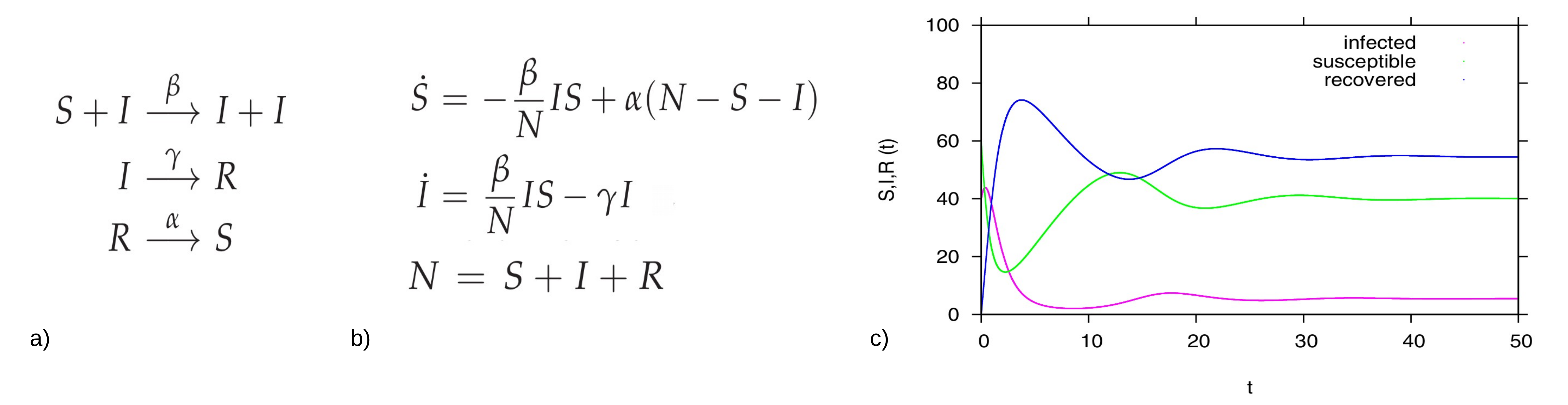
Figure 2: For the basic SIR type model, in a) reaction scheme, in b) ODE system and in c) time dependent solution simulation, with a population N=100 (for the interpretation in percentages), and starting values I=40, S=60 and R=0 we fixed β=2.5, α=0.1, and γ=1. In green the dynamics for the susceptible S(t), in pink the dynamics for the infected I(t) and in blue the dynamics of the recovered R(t).

2.1. The stochastic SIR epidemic model:

The stochastic SIR epidemic is modeled as a time-continuous Markov process to capture population noise. The dynamics of the probability of integer infected and integer susceptibles, while the recovered follow from this due to constant population size, can be give as a master equation [9] in the following form:

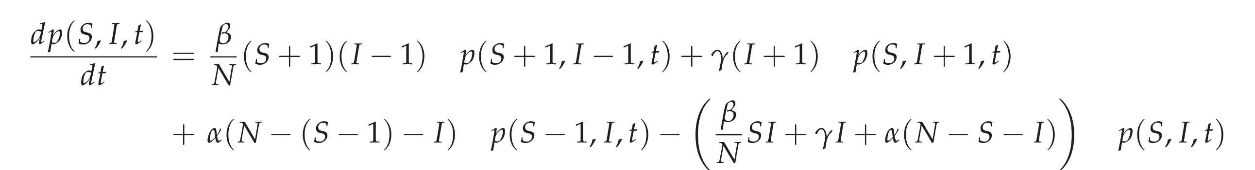
This process can be simulated by the Gillespie algorithm giving stochastic realizations of infected and susceptible in time [10,11]. The deterministic approach is obtained via the mean field approximation. For more details on the calculations see e.g. [12].

How does the program work: a short guide

Choose the parameters values for your simulation. Each susceptible individual is surrounded by 8 neighbors. “P” defines the probability of infection for each iteration. “Population Immunity” defines how many susceptible people exist in the population, and “Mortality” refers to the disease induced death probability.

Color code: green cells represent susceptible individuals, red cells represent infected individuals, blue cells represent recovered and immune individuals, and black cells represent deceased individuals.
Interpretation:
When the simulation starts, susceptible individuals (green cells) become infected randomly and cells turn red. For each iteration, new infection might occur within the 8 neighbors, with probability “P” of infecting someone. For example, if P = 50%, on average each cell will infect 4 neighbors per iteration.
Individuals are infected during the “Infected Period” and become recovered and immune (blue cells). For disease induced death (black cells), infected cells have a probability of “dying” at each iteration given by 1 – (1 – μ)^ (1 / p), where μ is the mortality rate and p is the infected period.
Output: On the right hand side, model output in terms of time series, for each variable, susceptible, infected, recovered/immune and deceased.

3. The SHAR Modeling framework:

To distinguish between mild and severely infected cases, the SIR framework can be extended into the so-called SHAR model, see Equation system below, where H stands for individuals developing a severe form of the disease and likely being hospitalized, while A refers to infected individuals who are asymptomatic or have a mild form of the disease. This system includes two additional epidemiological parameters: the severity ratio η and the infectivity factor Φ.

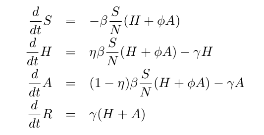
While the severity ratio η gives the fraction of infected individuals who develop severe symptoms (and hence 1-η gives the asymptomatic fraction of infections), the parameter Φ is a scaling factor used to differentiate the infectivity Φβ of mild/asymptomatic infections with respect to the baseline infectivity β of severe/hospitalized cases. The value of Φ can be tuned to reflect different situations: a value of Φ<1 reflects the fact that severe cases have larger infectivity than mild cases (e.g., due to enhanced coughing and sneezing), while Φ>1 indicates that asymptomatic individuals and mild cases contribute more to the spread of the infection (e.g., due to their higher mobility and possibility of interaction) than the severe cases which are more likely to be detected and isolated.

In the case of COVID-19, we assume Φ to be larger 1, since severe cases are likely hospitalized and isolated while mild/asymptomatic cases are often undetected and hence able to transmit the disease, contributing significantly more to the force of infection than the severe cases [13].

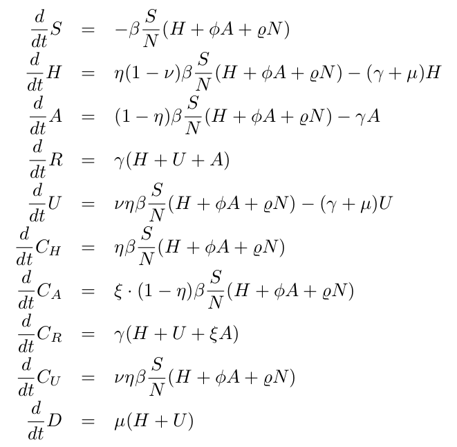
4. The SHARUCD model framework:

To model COVID19 dynamics, we use the SHARUCD framework, an extension of the simple SHAR model.

Here, “severity” is decided upon infection. While a proportion η of the individuals develop severe symptoms and are hospitalized, 1-η of the individuals would develop mild or asymptomatic infection. As severity progresses, a proportion ν would be admitted to an ICU facility. Hospitalized and ICU can recover or die (γ, μ ).

Similar to the basic SHAR assumptions, mild/asymptomatic infections are assumed to transmit the disease more efficiently (Φ>1) than severe/hospitalized cases.

As we investigate cumulative data on the infection classes and not prevalence, we also include classes C to count cumulatively the new cases (incidences) for “hospitalized” C_H, “asymptomatic” C_A, recovered C_R and ICU patients C_U. Note that C_A and C_R are depending on the detection rate ( ξ ) of positive
mild/asymptomatics.

The deceased cases are automatically collecting cumulative cases, since there is no exit transition form the death class D.

For completeness of the system and to be able to describe the initial introductory phase of the epidemic, an import term ρ should be also included into the force of infection.

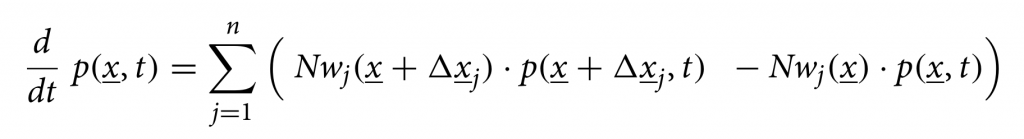
We consider primarily SHARUCD model versions as stochastic processes in order to compare with the available data which are often noisy and to include population fluctuations, since at times we have relatively low numbers of infected in the various classes. The stochastic version can be formulated through the master equation in application to epidemiology in a generic form using densities of all variables x1:=S/N , x2:=H/N, x3:=A/N , x4:=R/N , x5:=U/N , x6:=CH/N, x7:=CA/N , x8:=CU/N and x9:=D/N and x10:=CR/N, hence state vector x := (x1,…,x10)tr, giving the dynamics for the probabilities p(x,t) as

For a more detailed description of the SHARUCD model framework, see [13,14]. The SHARUCD model is able to describe the dynamics observed for PCR tested positive cases, hospitalizations, intensive care units (ICUs) admissions, deceased and finally the recovered. Keeping the biological parameters for COVID-19 in the range of the recent research findings, but adjusting to the phenomenological data description, the models were able to explain well the exponential phase of the epidemic and fixed to evaluate the effect of the imposed control measures. With good predictability so far, consistent with the updated data, we continued this work while the imposed restrictions were relaxed, closely monitoring the disease spreading dynamics.

The deterministic approach is obtained via the mean field approximation of the stochastic system, see below the ODE system for all classes, and is also used to evaluate the model performance and accuracy to guide the modeling analysis. The models are calibrated using the empirical data for the Basque Country and the biological parameters are either estimated or fixed as the model is able to describe the disease incidence data.

Note: The original version of the SHARUCD model the ICU admissions were assumed to be a progression to deceased. Due to the observed synchronization of transitions to hospitalization and asymptomatic cases (see section 4.4), the model was refined, changing the transition into ICU admissions to a ratio, analogously to the ratio for hospitalizations [15].

4.1. Modeling the effects of the control measures (First phase):

With the initial parameters estimated and fixed on the exponential phase of the epidemic, we model the effect of the disease control measures introduced using a standard sigmoid function σ(x)=1/(1+ex) . This function was able to describe well the gradual slowing down of the epidemics, as it turned out later in the response of the disease curves to the control measures. The current SHARUCD framework evaluates the seasonal effect on COVID-19 dynamics in the Basque Country, after social distancing measures start to be lifted (from May 4 – phase 0 and from May 11 -phase 1 towards the “new normality”). Model simulations with a single parameter set include now 2 control functions, shown in Fig. 3: one for the lockdown implementation and a second one for gradual lockdown lifting. Low seasonality is assumed to play a role, helping to keep transmission at low levels (see Fig. 5).

The seasonal forcing is implemented as a simple cosine function

β(t)=β0 (1+ θ cos(ω(t+φ))) on top of the already implemented sigmoidal control function σ(x)=1/(1+ex) from what we obtain the final format β(t)=β0 σ–(x) + β1 σ+(x) σ–(x1) + β2 σ+(x1 ) with σ–=1/(1+ex); σ+=1/(1+e-x); x=a(t-tc) and x1= a1(t-tc1).

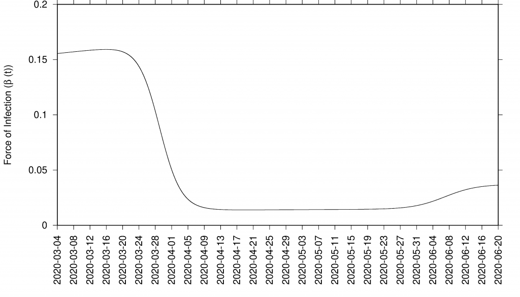
Figure 3: Sigmoid function as effect of control measures in infection rate β = β (t)

4.2. Model simulations with control and data:

The results presented here were obtained using two control functions described above and shown in see Fig. 3. Although still difficult to disentangle the possible seasonal effect from the draconian social distancing measures implemented during the lockdown, the SHARUCD model is unable to describe the most recent data without assuming low seasonal effect, showing a considerable overestimation of hospitalizations and deceased cases by assuming differences in transmission rate restricted to the social behaviour only.

In good agreement, the refined model can describe well the hospitalizations, the ICU admissions and the deceased cases, well matched within the median of the 200 stochastic realizations (incidences are shown in Fig. 4 and cumulative cases are shown in Fig. 5). The cumulative incidence for all positive cases follows the higher stochastic realizations range and the deviation observed between model simulations and data can be explained by the increasing testing capacities since March 22, 2020, followed by the introduction of rapid tests, mostly used as screening tools in nursing homes and public health workers. The current model (without testing feedback) can not describe this variable quantitatively, and would need further refinements and parametrization. The cumulative incidences for alive hospital discharges (black dots), used as a proxy for notified COVID-19 recovered individuals who were hospitalized, keeps following the lower realizations range when model simulations are obtained for the cumulative notified recovered (H+U+ξA), shown in Fig. 5 e) Figure 5 f) shows model simulations obtained for the cumulative notified recovered from hospital (H+U) only. A new transition is needed to record a proportion of recovered individuals tested positive without being admitted to the hospital (χA) in order to describe quantitatively describe the available data.

Figure 4: SHARUCD Model validation from March 4 to June 30 (incidences) Data are plotted as black line. The mean of 200 stochastic realizations are plotted as a blue line. The 95% confidence intervals are obtained empirically from 200 stochastic realizations and are plotted as purple shadow.

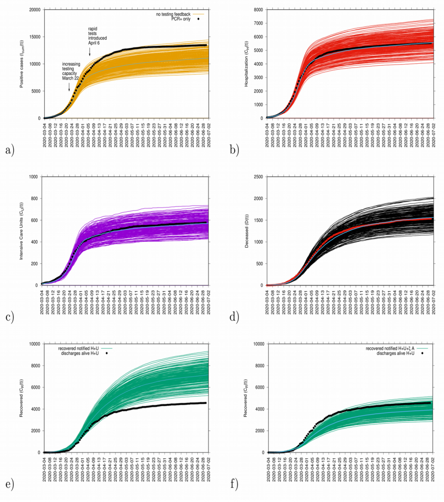
Figure 5: Ensemble of stochastic realizations of the refined SHARUCD-model. Model validation via data matching from March 4, 2020 to June 30, 2020. In a) cumulative tested positive cases Icum(t) (PCR+ only), b) cumulative hospitalized cases CH (t), c) cumulative ICU admissions CU(t), and d) cumulative deceased cases D (t). Using data for “hospital discharges alive”, we match in e) the simulations for the cumulative notified recovered CR(t) for H+U+ξA. In f) we plot the simulations for the cumulative notified recovered CR(t) for H+U only.

4.3. Model Validation and short-term prediction exercise with control measure:

Model validation and short-term predictions considering the effective control measures described above are shown in Fig. 6. For this exercise, empirical data available up to June 30, 2020, and model simulations are obtained for a four weeks longer run than the available data. New data will be included to check the quality of the short prediction exercise.

Figure 6: Mean and the 95% CI for the ensembles of stochastic realizations of the SHARUCD-model with control and data matching, starting from March 4, 2020. In a) cumulative tested positive cases Icum(t) (PCR+ only), b) cumulative hospitalized cases CH(t), c) cumulative ICU admissions CU(t), and d) cumulative deceased cases D (t). Using data for “hospital discharges alive”, we match in e) the simulations for the cumulative recovered CR(t) for H+U+ξA and in f) we plot the simulations for the cumulative recovered CR(t) for H+U only.

4.4. Growth rate and reproduction ratio:

The initial exponential growth rate λ of an epidemic is an important measure that follows directly from data at hand, commonly used to infer the basic reproduction number r, often called R0. While the momentary growth rate follows directly from the time continuous data at hand (see Fig. 7), the momentary reproduction ratio depends on the notion of a generation time γ-1.

Figure 7: Growth rate estimation from the data on all PCR positive tested cases for various variables: tested positive cases in yellow, hospitalizations in red, ICU admissions in purple, hospital discharges alive (proxy for recovered) in green and deceased in black.

The momentary growth rates and momentary reproduction numbers for the tested positive cases are calculated using data at hand available, from March 4 to June 39, 2020, shown in Fig. 8 a-b). Fig. 8 c) shows the behavior of the three synchronized variables, Icum, CH, and CU, crossing the threshold to a negative growth rate on April 1st, 2020, confirming the observed r(t) trend obtained by looking at data on Icum alone. Fig. 8 d) shows the synchronization of recovered and deceased cases, following toward the negative growth rate 1-2 weeks later, due to the delay between onset of symptoms, hospitalization and eventually death, reaching negative growth rate on April 7 and April 11, 2020, respectively. These results led to information about how to refine the model in order to capture the dynamics of the ICU admissions, better than in the original model, described in section 4.

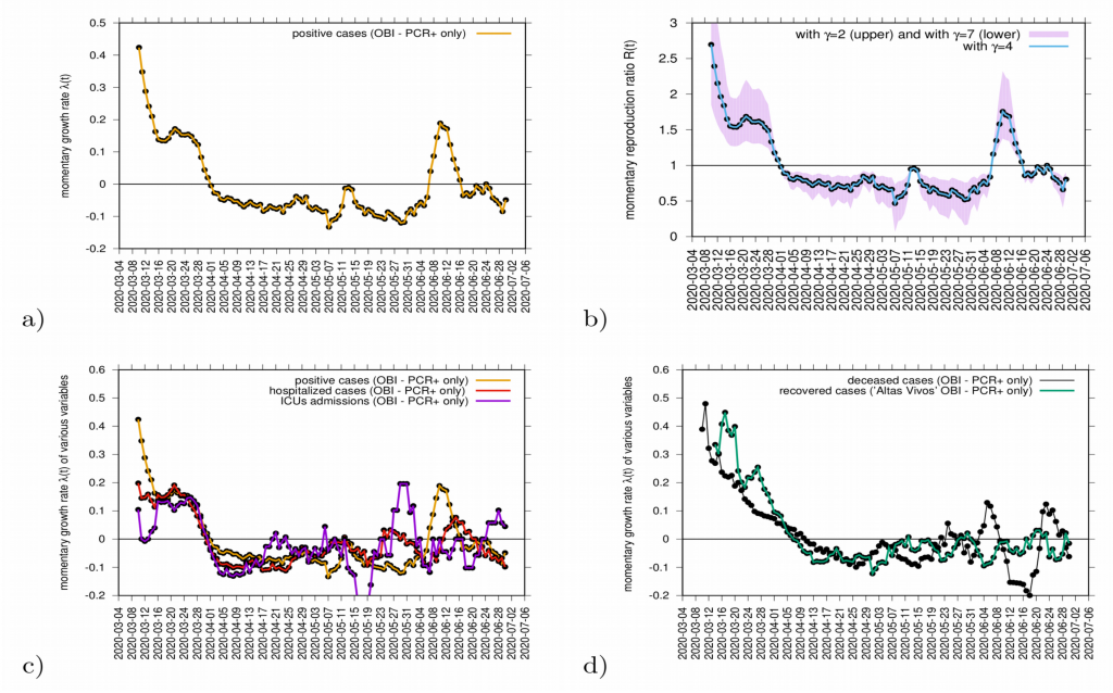
Figure 8: a) Growth rate estimation from the data on positive tested infected cases, and b) reproduction ratio from the same data, with different recovery periods. In c) combined growth rate for tested positive cases (yellow), hospitalizations (red) and ICU (purple) and in d) combined growth rate for recovered (green) and deceased (black). Clearly, the two groups can be distinguished.

Although the absolute value of r(t) can vary given the modeling assumptions considered during its estimation, it is advised to rather look at the threshold behavior, using the growth rates primarily as it is independent of modeling uncertainties and clearly indicates if the outbreak is under control or not when estimations are below or above threshold.

The growth rates for the tested positive cases have oscillated, crossing the threshold in middle June when some isolated outbreaks were identified and controlled. At the moment, the growth rate is negative, indicating a decrease of transmission. The reproduction ratio r(t) is also estimated to be below the threshold behavior of r=1, and careful monitoring of the development of the outbreak is needed. Important to note that the increased testing capacity allows the identification of mild/asymptomatic cases, is influencing the reproduction ratio behaviour.

Complementary measures of growth rates, shown in Fig. 9, for different variables such as hospitalization, intensive care units (ICU) admissions and deceased, can be also evaluated as data is consistently collected and defined. The evaluation of those measures together balance the interpretation of the behaviour of disease transmission in the Basque Country (see Fig. 9).

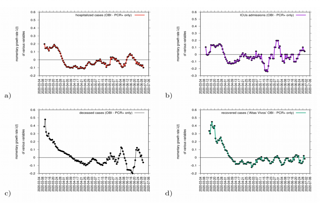
Figure 9: Growth rate estimation for various variables. In a) hospitalizations (red) and in c) ICU admission cases (purple). In c) growth rate for recovered (green) and in d) deceased (black).

5. The refined SHARUCD MODEL with import and seasonality (Second phase):

The current SHARUCD framework evaluates the seasonal effect on COVID-19 dynamics in the Basque Country, after social distancing measures start to be lifted (from May 4 – phase 0 and from May 11 -phase 1 towards the “new normality”). An import factor is also included in the model dynamics, after the full lockdown lifting in July. Although this factor was not important during the exponential growth phase, imported infections play a major role when small numbers are detected (stochastic phase pre/post exponential phase). It refers to infected individuals (most likely asymptomatic) coming from outside the studied population (either an infected foreigner visiting the region or an infected Basque returning to the country and that are not detected by the current testing strategy.)

Note that when the community transmission is under control (social distancing, masks and hygienic measures), the import factor does not contribute significantly to the epidemic, only starting isolated outbreaks (variable sizes depending on the momentary infection rate), but not driving the current epidemic into a new exponential growth phase.

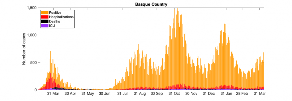
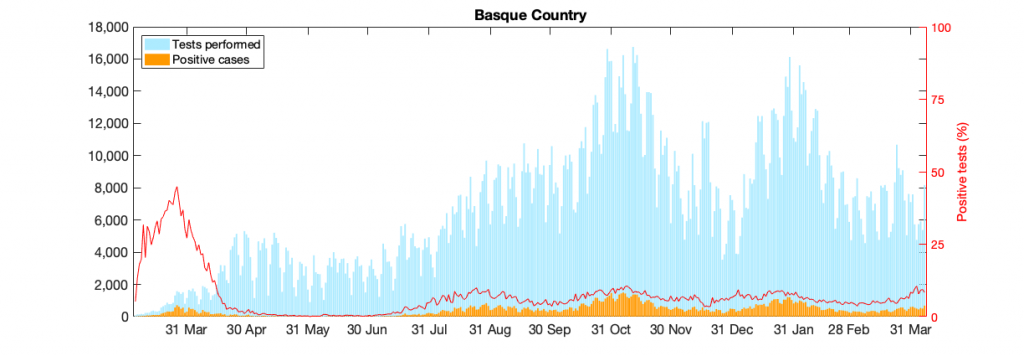
Figure 10: Figure 10: In a) COVID-19 in the Basque Country figure From March 4 to April 7, 2021, positive PCR cases (in yellow), Hospitalizations (in red), ICU admission (in purple) and deceased cases (in black) are shown. In b) COVID-19 tests performed in the Basque Country (in light blue) and positivity rates (red line).

5.1 Model simulations and short term predictions:

The model shown in section 4 analyses now isolated outbreaks (assuming now import to asymptomatic infection) after lifting of lockdowns and increased detection of asymptomatic due to now intensified contact tracing with time dependent infection rate β, and now also increased import ρ and increased detection of asymptomatic cases ξ over time.

Model parametrization is now also considering the detected positive cases data, in order to disentangle the role of import ρ from community spreading β. From September 15 onwards the daily testing capacity is varying significantly, however the cumulative positivity rates are stabilized (≈ 6.3%). The model predicts an endemic state for positive cases and it is, at the moment, overestimating the mean of positive cases detected using PCR tests. That is because the current assumed detection rate parameter has decreased (and keeps varying) and must be adjusted. More tests would eventually identify those asymptomatic cases predicted by the model, as observed in the last few days with the number of tests increasing significantly. Antigen tests were introduced on Oct. 17, 2020, with an important increase in testing capacity (See Fig. 10b)).

As the trend of stationarity continues with import cases (i.e. non detected asymptomatic infections) possibly causing isolated outbreaks, the community transmission is below the threshold, i.e controlled and not increasing to a new exponential phase in the next few days. Note that on October 27, a new lockdown was implemented and transmission rate has decreased even more. Although the trend of stationarity does not appear to be changed, a new control function was included in order to describe the current epidemiological scenario of decreasing detected positive cases.

5.2 Short term predictions of COVID-19 in the Basque Country:

Cumulative cases:

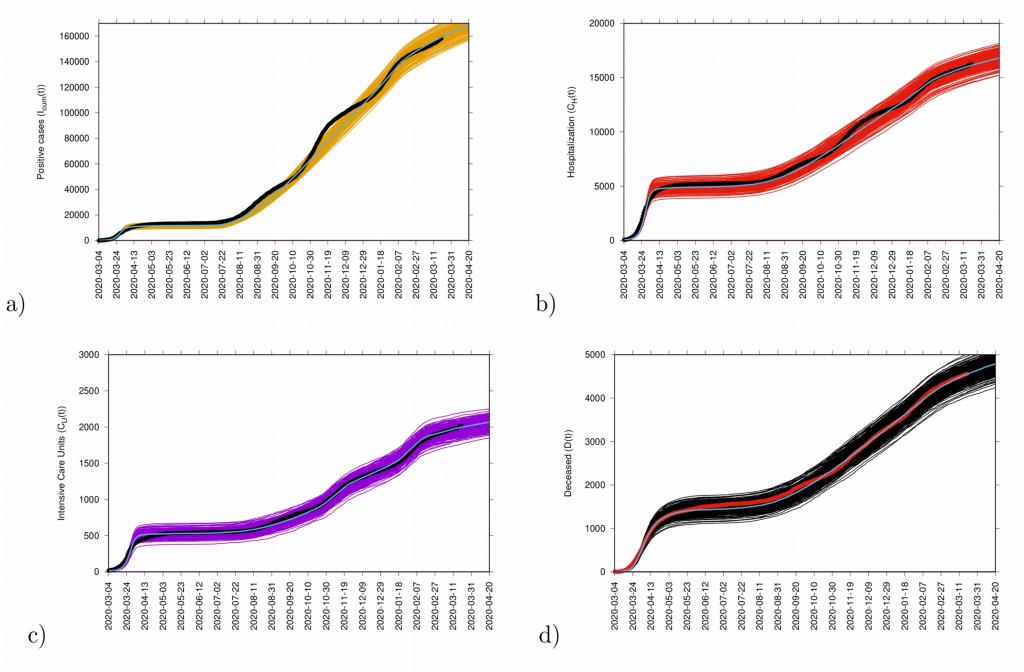
Figure 11: Ensemble of stochastic realizations of the refined SHARUCD-model with import. In a) cumulative positive cases I cum (t), in b) cumulative hospitalized cases C H (t), in c) cumulative ICU admissions C U (t) and in d) cumulative deceased cases D(t). The mean of 500 stochastic realizations are plotted as a blue line._

Incidence cases:

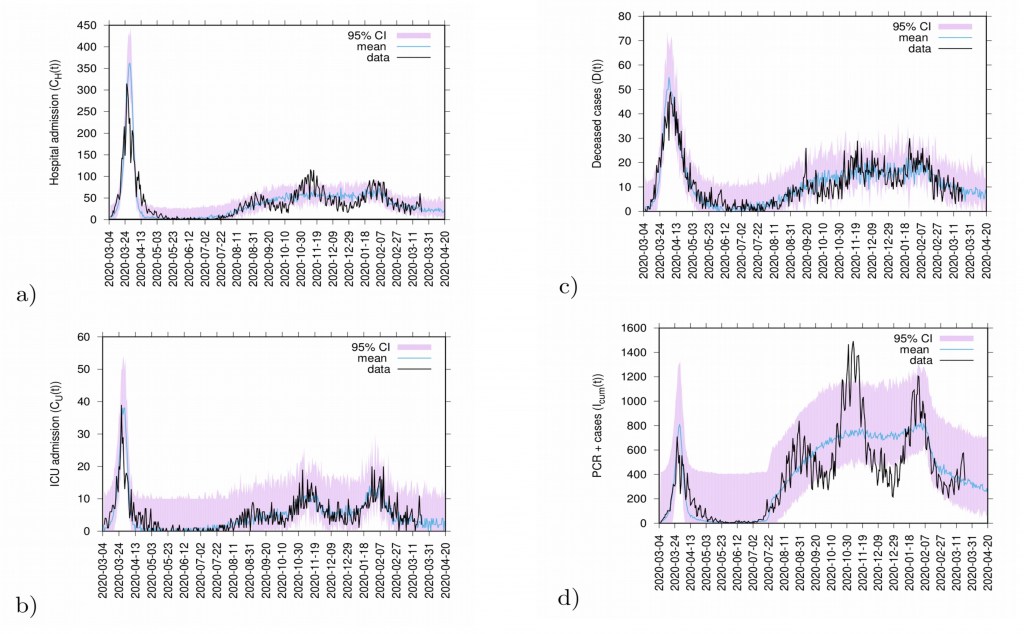
Figure 12: 20 days predictions. In a) hospitalizations and in b) ICU admission. In c) deceased cases and in d) detected PCR positive cases.

Predictions are made with the refined SHARUCD model parameterized with empirical data described above. Deceased cases are estimated from the current data referring to detected positive cases and severe cases prone to hospitalization and are possibly been overestimated by the model (as PCR method can identify nucleic acid from the virus but can not differentiate between active or residual viral particles). Model predictions are shown as light blue curves. The 95% confidence intervals (CI) are plotted in light purple (shadow). Empirical data are plotted on top of the prediction curve in black.

6. Acknowledgments and contribution:

Maíra Aguiar, BCAM – Ikerbasque, MTB research line leader & University of Trento Marie Curie Fellow (COMPLEXDYNAMICS-PHIM Marie Skłodowska-Curie grant agreement No 792494): conceived the study, developed and analyzed the models.

Nico Stollenwerk, BCAM, MTB Group: developed and analyzed the models.

Nicole Cusimano, BCAM – MTB Postdoctoral researcher: data collection, analysis and graphical illustration.

Damián Knopoff, BCAM – MTB Postdoctoral researcher: data collection, analysis and graphical illustration.

Akhil Kumar Srivastav, BCAM – MTB Research Technician: data collection, analysis and graphical illustration.

Carlo Estadilla, BCAM – MTB PhD Student: data collection, analysis and graphical illustration.

Bruno V. Guerrero B., BCAM – MTB Research Technician: dashboard updates and followups.

Francisco P. Rodrigues, student at Instituto Superior Técnico, University of Lisbon, Portugal, has developed the SIR simulation program.

Eduardo Millán, Osakidetza Basque Health Service, has collected and prepared the data sets for COVID-19 incidences in the Basque Country. The data was used to calibrate the SHARUCD modeling framework.

Oliver Ibarrondo, Osakidetza Basque Health Service, has collected and prepared the data sets for COVID-19 vaccination in the Basque Country. The data was used to calibrate the SHARV modeling framework

We thank the huge efforts of the whole COVID-19 BMTF, specially to Joseba Bidaurrazaga Van-Dierdonck, Public Health, Basque Health Department, Javier Mar, Biodonostia Health Research Institute and Adolfo Morais Ezquerro, Vice Minister of Universities and Research of the Basque Government, for the fruitful discussions.

7. References:

[1] World Health Organization. Emergencies preparedness, response. Novel Coronavirus – China.

[2] World Health Organization. WHO announces COVID-19 outbreak a pandemic.

[3] WHO Coronavirus Disease (COVID-19) Dashboard

[4] European Medicines Agency.

[5] European Commission. Safe COVID-19 vaccines for Europeans

[6] COVID-19 Data Repository by the Center for Systems Science and Engineering (CSSE) at Johns Hopkins University

[7] Maíra Aguiar, Nico Stollenwerk and BobW. Kooi. (2012). Modeling Infectious Diseases Dynamics: Dengue Fever, a Case Study. Chapter In book: Epidemiology Insights.

[8] Fred Brauer. (2005). The Kermack–McKendrick epidemic model revisited. Mathematical Biosciences, 198(2), 119-131.

[9] van Kampen, N. G. (1992). Stochastic Processes in Physics and Chemistry, ISBN 978-0-44452-965-7. (North-Holland, Amsterdam).

[10] Gillespie, D.T. (1976). A general method for numerically simulating the stochastic time evolution of coupled chemical reactions. Journal of Computational Physics, 22, 403-434, ISSN 0021-9991.

[11] Gillespie, D.T. (1978). Monte Carlo simulation of random walks with residence time dependent transition probability rates. Journal of Computational Physics, 28, 395-407, ISSN 0021-9991.

[12] Stollenwerk, N. and Jansen, V. (2010). Population biology and criticality, ISBN 978-1-84816-401-7. (Imperial College Press, London).

[13] Aguiar, M., Ortuondo, E.M., Bidaurrazaga Van-Dierdonck, J. et al. Modelling COVID 19 in the Basque Country from introduction to control measure response. Nature Scientific Reports 10, 17306 (2020).

[14] Aguiar, M. and Stollenwerk, N. SHAR and effective SIR models: from dengue fever toy models to a COVID-19 fully parametrized SHARUCD framework. Commun. Biomath. Sci. 3(1), 60–89 (2020).

[15] Aguiar, M., Van-Dierdonck, J. B. and Stollenwerk, N. (2020). Reproduction ratio and growth rates: measures for an unfolding pandemic. PLoS ONE 15(7), e0236620.

[16] Aguiar, M. and Stollenwerk, N. (2020). Condition-specific mortality risk can explain differences in COVID-19 case fatality ratios around the globe. J. Public Health, 188, 18-20.

[17] Aguiar, M., Van-Dierdonck, J.B., Mar, J. et al. (2021). Critical fluctuations in epidemic models explain COVID-19 post-lockdown dynamics. Nature Scientific Reports, 11: 13839.

[18] Maíra Aguiar, Joseba Bidaurrazaga Van-Dierdonck, Javier Mar, Nico Stollenwerk (2021). The role of mild and asymptomatic infections on COVID-19 vaccines performance: a modeling study. Journal of Advanced Research (in press).

[19] Maíra Aguiar, Vizda Anam, Nicole Cusimano, Damián Knopoff and Nico Stollenwerk. (2022). Understanding COVID-19 epidemics: a multi-scale modeling approach in Predicting Pandemics in a Globally Connected World, Volume 1 – N. Bellomo and M. Chaplain, Eds., Birkhäuser-Springer Series “Modeling and Simulation in Science, Engineering and Technology”, to appear.

[20] Maíra Aguiar, Giovanni Dosi, Damián A. Knopoff and Maria Enrica Virgillito (2021). A multiscale network-based model of contagion dynamics: heterogeneity, spatial distancing and vaccination, Mathematical Models and Methods in Applied Sciences.

Table of contents: